Figure S7:
Files in tutorial_input_files.zip necessary to reproduce the results in Fig. 6 of the main text (part 1/2). By executing the command ./FIG6.sh (or ./FIG6.sh X, with X the number of parallel processes), all the results of Fig. 6 can be obtained and the figure can be plotted.
The background colors indicate whether it is a folder (green), an input file (purple), an executable (yellow), or an explanation (white). Here, SSI is short for single-shot images. The input files analysis2.inp are used for generating
 at
at  for the supplementary movie. They should be renamed as analysis.inp when used. The input files can be downloaded at http://ultracold.org/data/tutorial_input_files.zip.
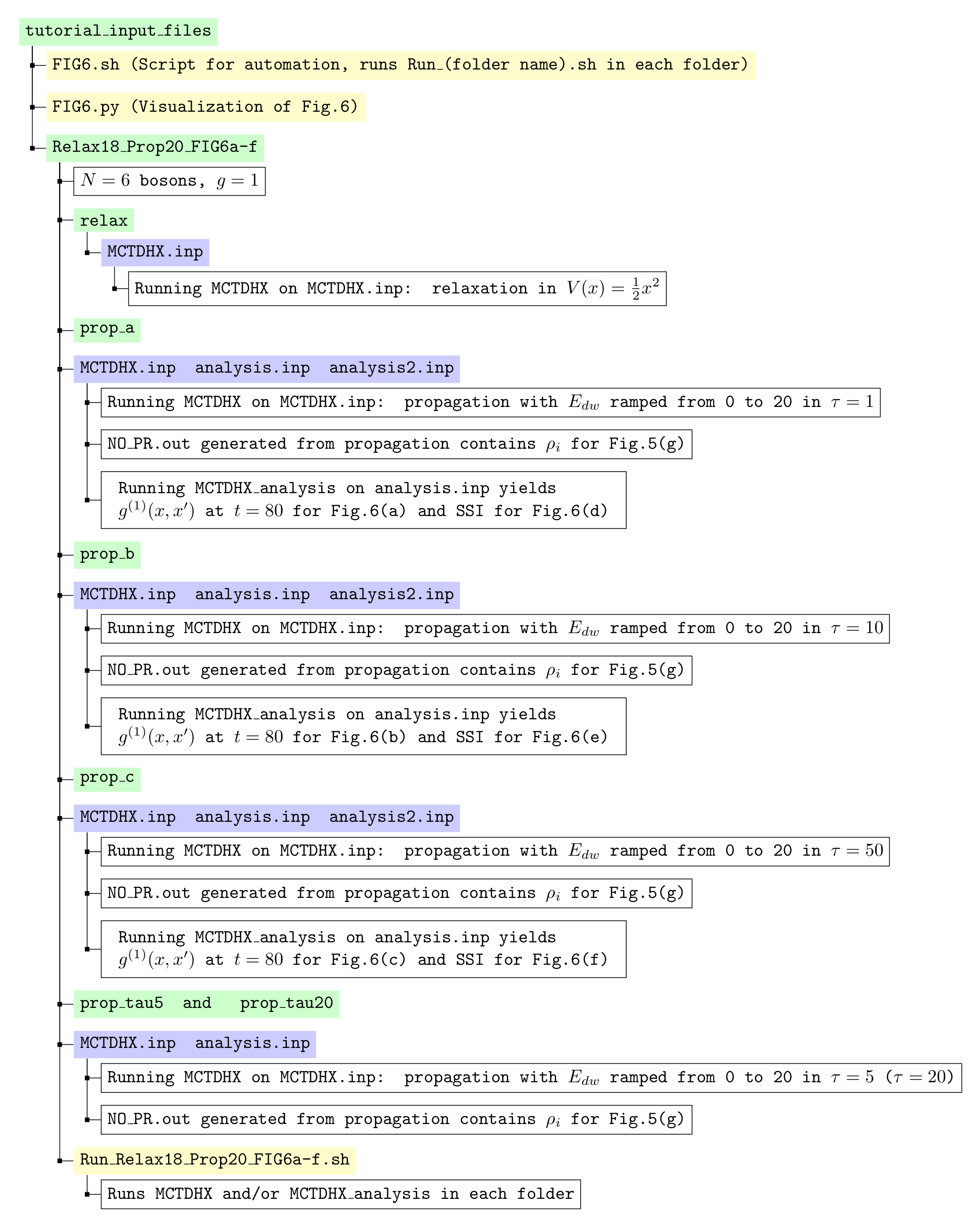 |
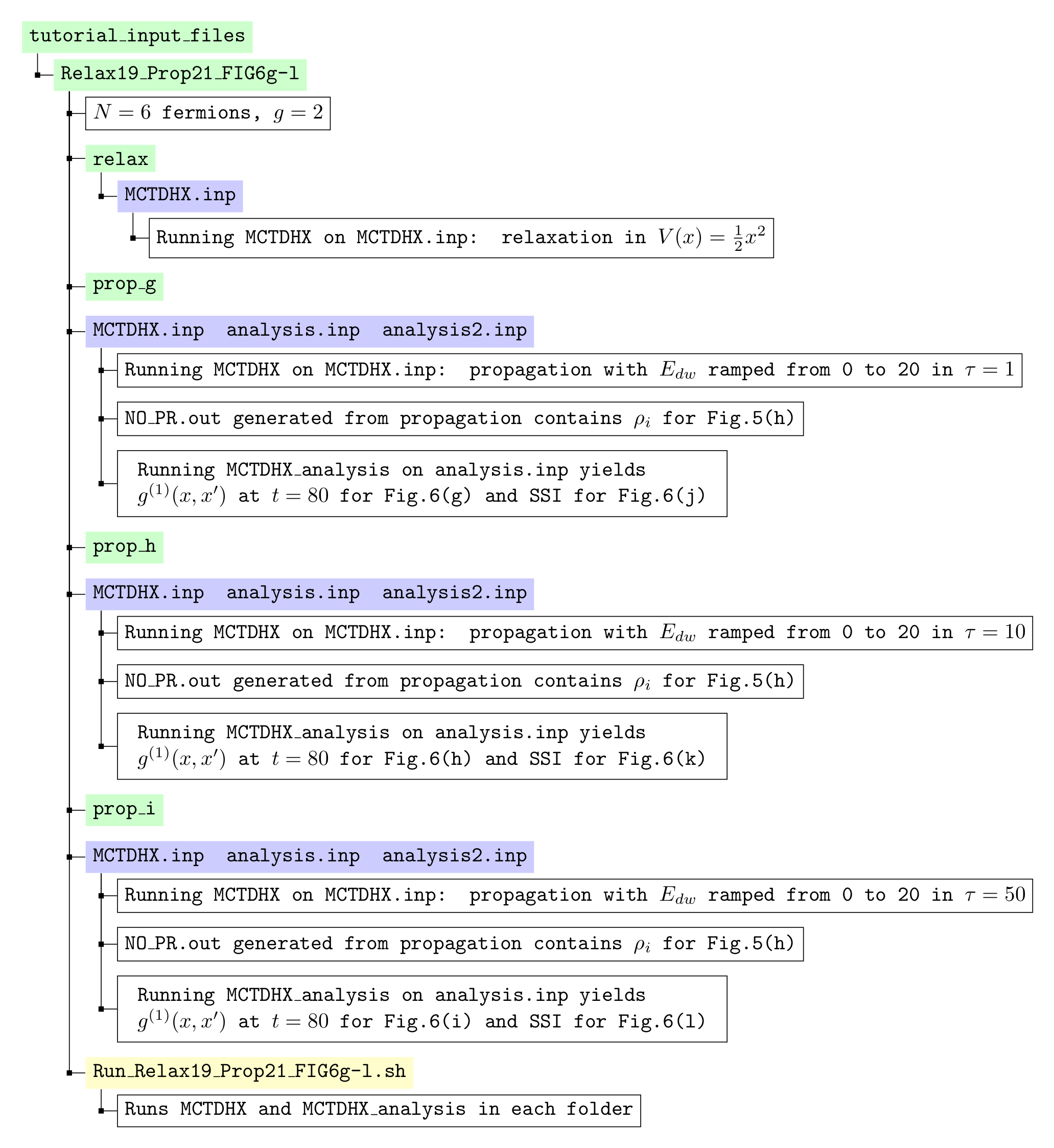
Figure S8:
Files in tutorial_input_files.zip necessary to reproduce the results in Fig. 6 of the main text (part 2/2). By executing the command ./FIG6.sh (or ./FIG6.sh X, with X the number of parallel processes), all the results of Fig. 6 can be obtained and the figure can be plotted.
The background colors indicate folders (green), input files (purple), executables (yellow), and explanations (white). Here, SSI is short for single-shot images. The input files analysis2.inp are used for generating
at for the supplementary movie. They should be renamed as analysis.inp when used. The input files can be downloaded at http://ultracold.org/data/tutorial_input_files.zip.
 |